Google Sheets IF-THEN Formula

Understanding Functions in Google Sheets

Functions are an inevitable part of working with spreadsheets. 

A function is a predefined formula that performs calculations using specific values, called arguments, in a particular order. They can be used to perform various operations such as summing up cells, counting the number of characters in a cell, or finding the average of a range of cells.

Google Sheets support 2 types of functions: built-in and custom functions.

1. Built-in functions are the most commonly used type of function. They’re already programmed into Google Sheets and ready to use.
2. Custom functions are created by users (like you and me!) using Google Apps Script, a scripting language based on JavaScript.

The most important thing to know about functions is how to use them. In general, you’ll use a function by typing = (equal sign) followed by the function name and its arguments.

The function name is the name of the action you want to perform. The arguments are the values or cell references that tell the function what to work on.

For example,  the sum function adds up a range of cells. The syntax for the sum function is =sum(range).

In this example, “range” is the argument that tells the function of the cells to add up.

You can also use more than one argument in a function.

Out of all the functions, the IF-THEN function is probably the most versatile. It allows you to automate tasks based on certain conditions.

What is the Google Sheets IF-THEN formula

The IF-THEN function is also known as the conditional formatting function or IF-THEN formula.

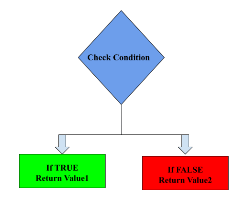
It is like a decision tree where the result will be one of the two outcomes, based on the conditions you set.

Here’s the syntax for it

=if(condition, value if true, value if false)

Here,

• condition is the criteria that you want to test.
• value if true is the value returned if the condition is satisfied
• value if false is the value returned if the condition is not satisfied. The value_if_false argument is optional, but I recommend always including it. That way, you can control what happens when the condition is met and when it’s not.

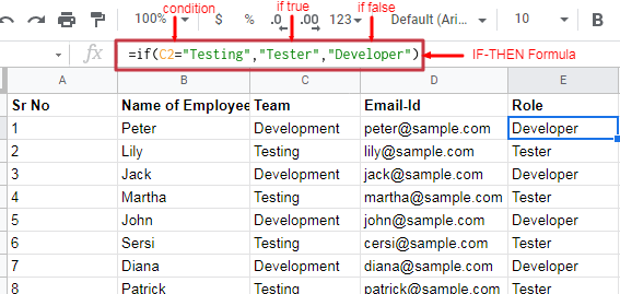
For example, we can set the role to Developer/ Tester based on a condition that checks whether the department of the employee is ‘Testing’ as shown below.

Now that we’ve gone over the basics of how the IF-THEN formula works, let’s look at some more examples of how you can use it.

Examples of How to Use Google Sheets IF-THEN Formula

Here are some examples of how you can use the IF-THEN function in Google Sheets.

Format Numbers as Currency:

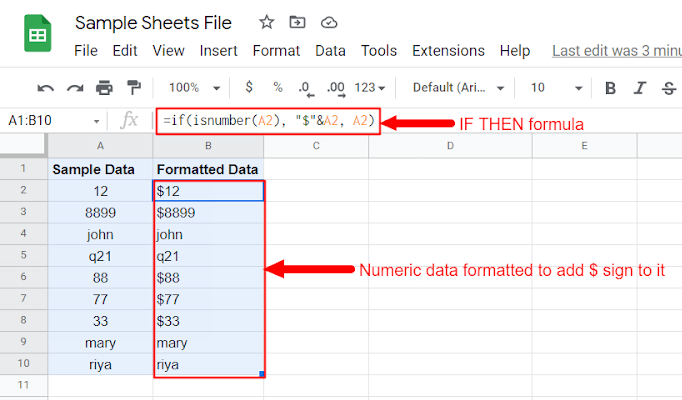
You can use the IF-THEN function to automatically format numbers as currency. To do this, you’ll need to use the condition of whether or not a cell contains a number. And if it does then use the “$” symbol to format the cell as currency. And in case it’s not a number then leave the cell as it is.

Here’s what the final formula looks like:

=if(isnumber(A), “$”&A, A)

Find out the Expired Dates:  

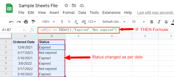
You can use the IF-THEN function to find out the expired dates. To do so, use the condition: whether or not a date has expired and set the status to ‘Expired’ or ‘Not Expired’ accordingly Here’s what the final formula looks like:

=if(A <= today(), “Expired”, “Not Expired”)

Perform calculations: 

In scenarios where you need to perform calculations based on some decisions, you can again opt for IF-THEN formula. For example, if you want to offer discounts to your customers based on the amount of purchase, you can use IF-THEN to calculate the discount amount and show it in a separate column. For example, assume that you own a store and offer discounts to customers based on the amount of their purchase as:

• If a customer spends less than $100, they get a 15% discount. 
• If a customer spends between $100 and $199, they get a 20% discount, and
• If a customer spends $200 or more, they get a 25% discount.

Then you can use a formula like:

=if(A <= 100, 15%, if(A <= 199, 20%, 25%))

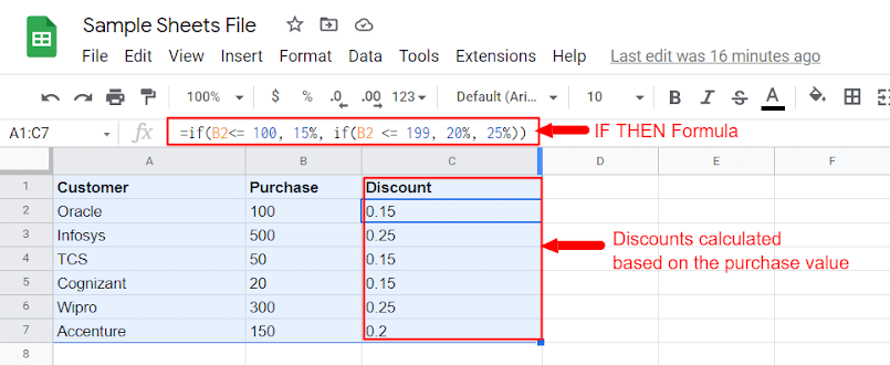
The format of IF used in the above formula is a NESTED IF.  Continue reading to understand what it is.

Nested IF-THEN

A nested IF-THEN statement is an “IF-THEN” statement that contains another “IF-THEN” statement. 

The syntax for it is as follows: 

=if(condition, value if true, if(condition, value if true, value if false))

In the above formula, the first “IF-THEN” statement has a condition and two values: one for when the condition is met and one for when it’s not. 

The second “IF-THEN” statement also has a condition and two values. However, the second “IF-THEN” statement is only executed if the first “IF-THEN” statement’s condition is not met. 

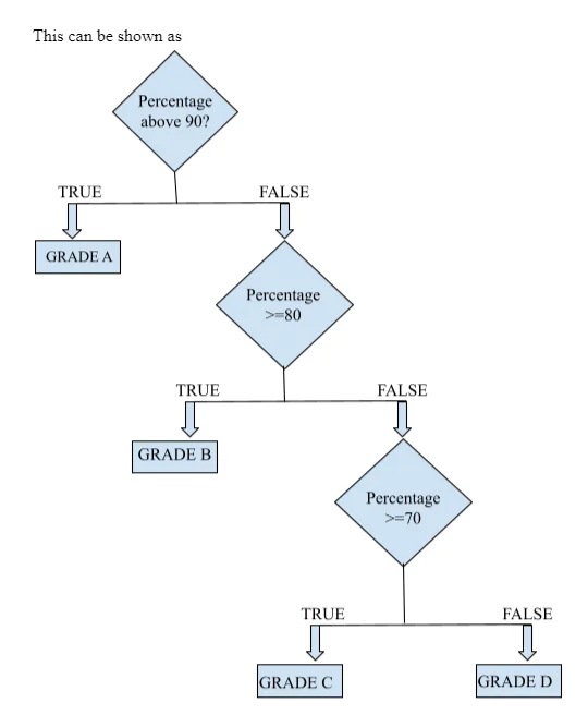
For example,  let’s say you want to grade students based on the following criteria: 

• A score of 90 or above,  Grade = “A”. 
• Score between 80 and 89, Grade = “B”. 
• Score between 70 and 79, Grade = “C”. 
• Score below 70, Grade = “F”. 

This can be shown as

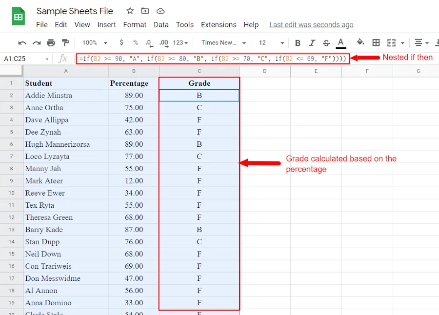
You can use the following nested “IF-THEN” statement to calculate the grade: 

=if(A >= 90, “A”, if(A >= 80, “B”, if(A >= 70, “C”, if(A <= 69, “F”))))

Using nested if can sometimes be very cumbersome as your conditions increase, IFS comes to your rescue at this point.

IFS function in Google Sheets

The IFS function is a newer way to do nested ifs, it was introduced in google sheets in 2018. IFS can take multiple conditions and return multiple results. Its syntax is as follows:

=IFS(condition_a, result_a, condition_b, result_b, …)

So for the above example, we can modify the condition to get the same result as:

 =IFS(A >= 90, “A”, A >= 80, “B”, A >= 70, “C”, A <= 69, “F”)

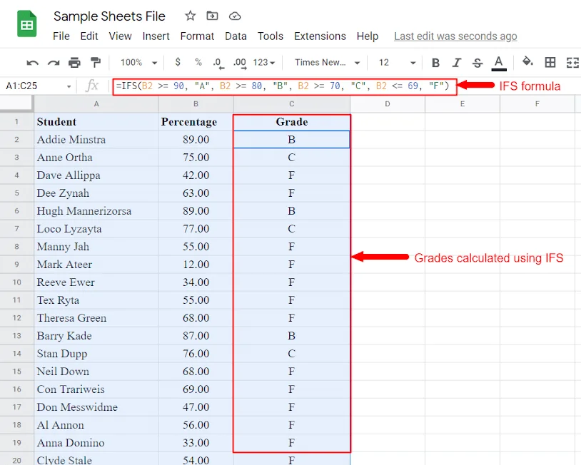
As you can see, the IFS function is much cleaner and easier to read than a nested IF statement.

That’s it for this tutorial! You should now have a good understanding of how to use the IF function in Google Sheets. So, automate all the tasks that you can and get relieved!

Don’t stop here, continue learning about all the different ways you can use Google Sheets by checking out our other tutorials.

Also, to further automate your workflow process, we have Integrately at your service!

Integrately is  an automation tool that lets you automate your apps like Google Sheets in just 1 click. That too with more than 700+ other apps.

Spend only a few minutes initially and be carefree afterward. No technical skills are required!

Save yourself lots of time & money.